How To Continue Numbering In Google Sheets
Then as in step 3 select the Number option. A blue box will appear around all of them.
How To Increment Number In Google Sheet How To Number Rows In Google Sheets Youtube
Then tap the specific number you want to change to select just that one.
How to continue numbering in google sheets. Learn how to fill automatically sequence of no in google sheet. Then select the formula cell and drag the fill handle down to the cells that you want to apply this formula and all numbers have been extracted from each cell as. Insert a column to the left the Name column.
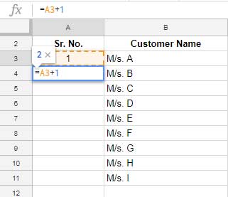
Next in step 2 you will go to the Format tab. In cell A3 enter 2. Built-in formulas pivot tables and conditional formatting options save time and simplify common spreadsheet tasks.
In cell A2 enter 1. First select the range of cells that you want to format. To pull Google Sheets data from another sheet use.
For these examples Im assuming I have numbers currency numbers percentages or dates in column A. Some text The second rule which comes between the first and second semi-colons tells Google Sheets how to display negative numbers. See the above screenshot.
In a column or row enter text numbers or dates in at least two cells next to each other. Suggestion - Pre-format the cells beforehand as shown in the picture below whereby you will first have to highlight the concerned column or cell. Click on the cell you want to format.
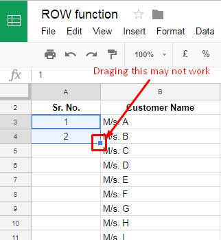
My GearCamera - httpamznto2tVwcMPTripod - httpamznto2tVoceRLens - httpamznto2vWzIUCMicrophone - httpamznto2v9YC5pLaptop - httpamznt. Dynamic Sequential Numbering in Google Sheets To generate serial numbers in a column that up to the value in the last row in another column we can use a Sequence Match function combination. Youll see a small blue box in the lower right corner.
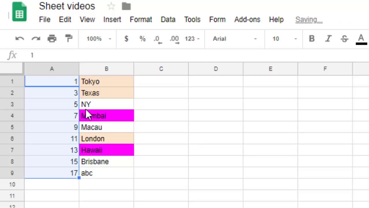
Using the fill handle to fill down numbers also work when you have some text along with the number. Here in this case in Cell A4 use the formula A31 and then copy and paste this formula to the cells down. To change the numbering in a list tap the numbers with your cursor.
Use curly brackets for this argument. Number Rows Using Fill Handle. Next go to Format Number.
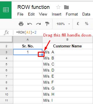
The first rule which comes before the first semi-colon tells Google Sheets how to display positive numbers. U can use Row or Row -1 or Row -i i can be any number. Drag the blue box any number.
This is commonly using the numbering method in Google or Excel spreadsheets. You can change the number formatting using the Format menu. Other way is to use Google script to number a range.
Use one of the formulas below. Select both the cells. Keep Leading Zeros as You Type If you want to keep a leading zero on the fly you can enter an apostrophe before you enter the number that begins with zero.
To format a cell to display more than two decimals not rounded up or down do the following. The apostrophe acts as an escape character and tells Sheets to ignore its programming that trims leading zeros. The easiest way is to use formula and then paste the formula in the range.
Format for negative numbers 000. You dont have to drag if you are using formula. Here youll see different formats like Number Percentage Scientific Accounting Financial Currency and Currency Rounded.
Google Sheets makes your data pop with colorful charts and graphs. Abcdefghijklmnopqrstuvwxyz into a blank cell where you want to extract the numbers only and then press Enter key all the numbers in Cell A2 have been extracted at once see screenshot. Auto Serial Numbering Using Simple Formula.
A1A3 Where A1A3 is the range of cells from your current active sheet. In case you use 1 and 3 in cell A2 and A3 respectively using the fill handle will give you a series of odd numbers as the pattern is to keep a difference of 2 in the numbers. Learn how to fill automatically sequence of no in google sheet.
Optional Give the new column a heading and format it like other columns. Combine Text And Numbers In Google Sheets To combine text in a cell or denoted by quotes Text and numbers use the TEXT function as shown in these examples. All for free.
SPLIT LOWER A2. Place your cursor in the cell where you want the referenced data to show up. To do this right-click on any cell in column A and select Insert Column.
Open a sheet in Google Sheets. And finally select the plain text option in step 4. To link data from the current sheet.
First see this normal formula that generates serial numbers 1. In the above example our serial numbering starts from row A3.

How To Number Rows In Google Sheets Add Serial Numbers Spreadsheet Point

Fill Down In Google Sheets Autofill Formulas Numbers Dates Spreadsheet Point
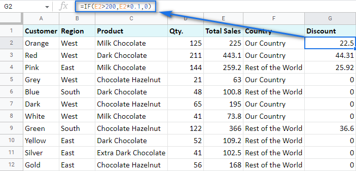
Google Sheets If Function Usage And Formula Examples

How To Sort By Number On Google Sheets On Pc Or Mac 7 Steps
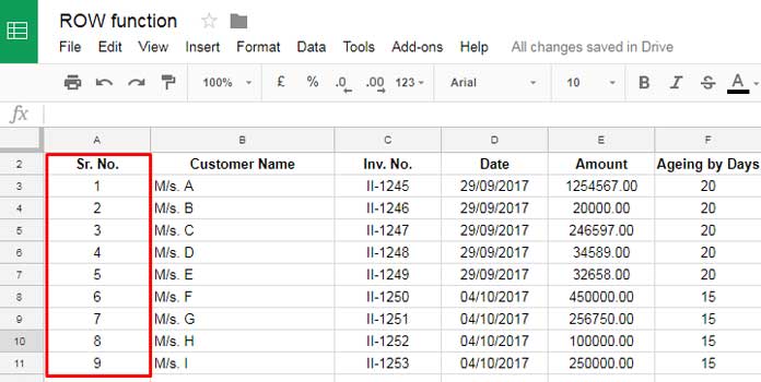
Auto Serial Numbering In Google Sheets With Row Function

Fill Down In Google Sheets Autofill Formulas Numbers Dates Spreadsheet Point

How To Number Rows In Google Sheets Add Serial Numbers Spreadsheet Point
Auto Serial Numbering In Google Sheets With Row Function

How To Subtract In Google Sheets With A Formula
Auto Serial Numbering In Google Sheets With Row Function

How To Sort By Number On Google Sheets On Pc Or Mac 7 Steps
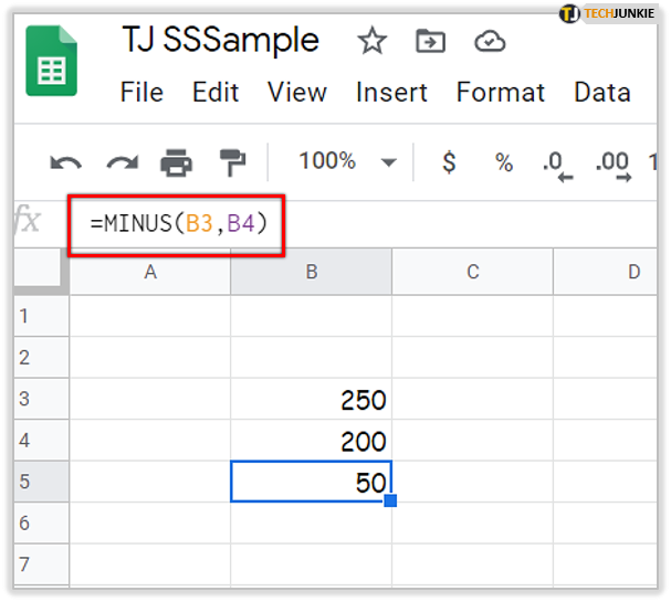
How To Subtract In Google Sheets With A Formula
/001-wrap-text-in-google-sheets-4584567-37861143992e4283a346b02c86ccf1e2.jpg)
How To Wrap Text In Google Sheets
Auto Serial Numbering In Google Sheets With Row Function
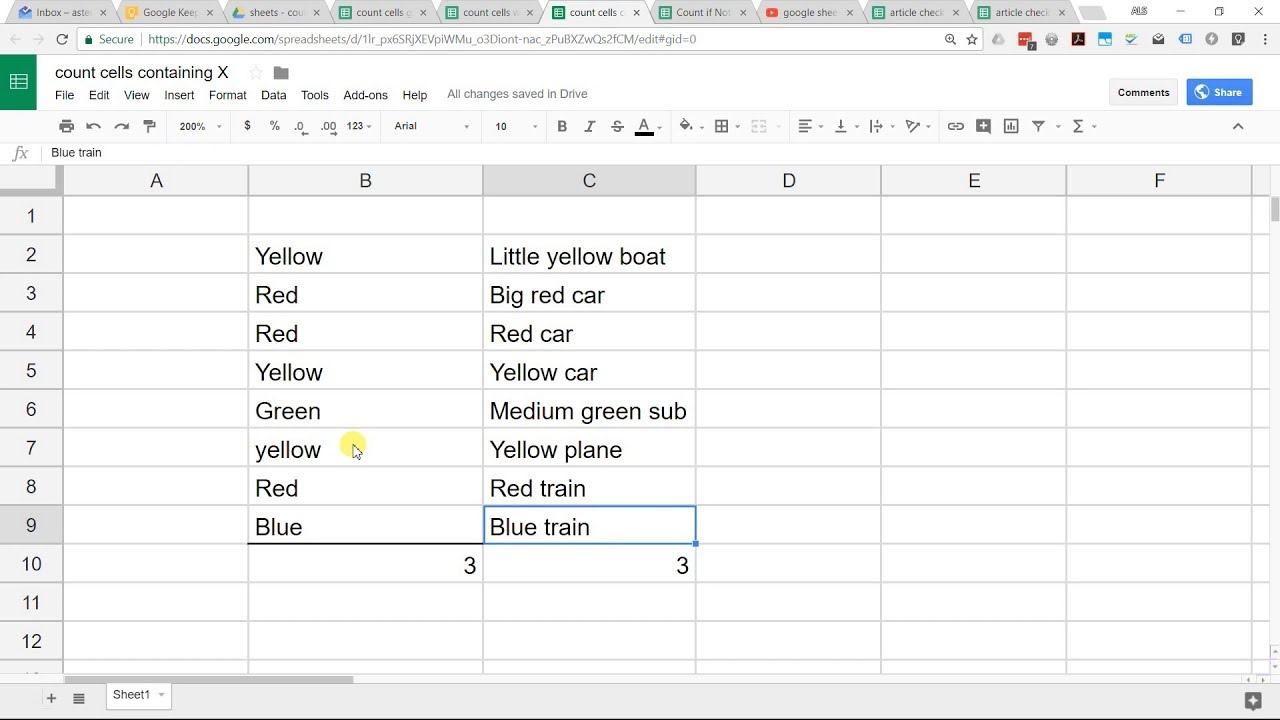
Google Sheets Count Cells Containing Specific Text Youtube

How To Number Rows In Google Sheets Add Serial Numbers Spreadsheet Point

How To Repeat The Top Row On Every Page In Google Sheets Solve Your Tech

Bullets And Numbering In Google Docs Youtube

Fill Down In Google Sheets Autofill Formulas Numbers Dates Spreadsheet Point