How To Put Number In Bar Chart Excel
Assuming youre using Excel 2007 data labels are added through the Data Labels selection. Once youve formatted your data creating a bar chart is as simple as clicking a couple buttons.

How Do You Put Values Over A Simple Bar Chart In Excel Cross Validated
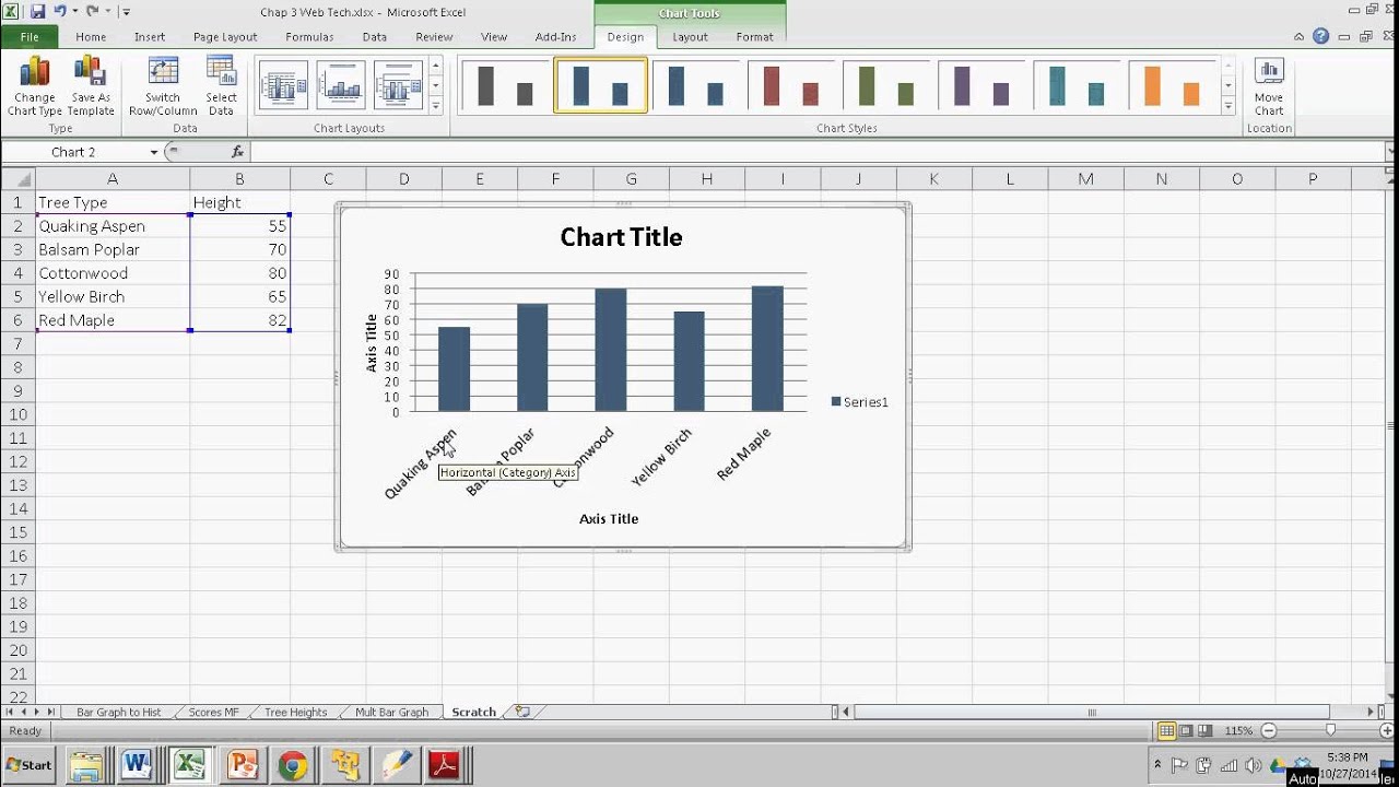
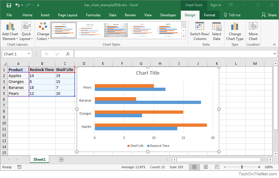
4 Click on the graph to make sure it is selected then select Layout.
How to put number in bar chart excel. The benefit of this method is that it also works with a 3D stacked bar chart. In the Charts section youll see a variety of chart symbols. Excel Data Bars Step 1.
Select data range you need and click Insert Column Stacked Column. By clicking on the title you can change the tile. You can do this manually using your mouse or you can select a cell in your range and press CtrlA to select the data automatically.
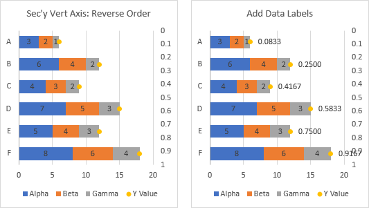
Formatting your Map chart. Add this series to the chart copy the cells with the numbers 1 to 5 select the chart use paste special and hit OK. Select series in chart.
The chart should look like this. Select the data and go to the chart option from the Insert menu. Make sure that AXIS OPTIONS is active at the right panel side.
B2115 and then drag the fill handle down to the cells see screenshot. In Sheet 2 you would insert a text box anywhere on the worksheet. In that text box you would type Sheet1A4 Move it to the top of the bar in the chart and voila all done.
In Excel 2007 click Layout Data Labels Center. Click on your ChartClick on the DESIGN tabClick on the QUICK LAYOUT 2nd from leftYou will find a number of layouts there to chose from. 1 Select cells A2B5.
Select the range with two unique sets of data then click Insert Insert Column or Bar Chart clustered column. Go to Insert and click on a Column chart. Right click format data series data labels label contains value.
After inserting the chart then you should insert two helper columns in the first helper column-Column D please enter this formula. To insert a bar chart in Microsoft Excel open your Excel workbook and select your data. Select the number range from B2 to B11.
Click at the column and then click Design Switch RowColumn. In the chart right-click the Series Footballers data series and then on the shortcut menu click Add Data Labels. First highlight the data you want to put in your chart.
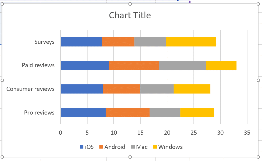
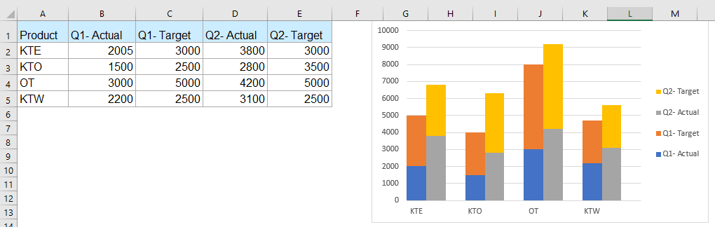
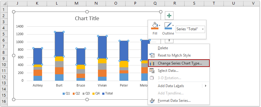
Select the specified bar you need to display as a line in the chart and then click Design Change Chart Type. 2 Select Insert 3 Select the desired Column type graph. Click on the bar chart select a 3-D Stacked Bar chart from the given styles.
One of the cool features is the ability to change number format in Excel chart. 2 go to INSERT tab click Bar command under charts group. To show text instead of the number labels on the X axis you need to add an additional series with the values 1 to 5.
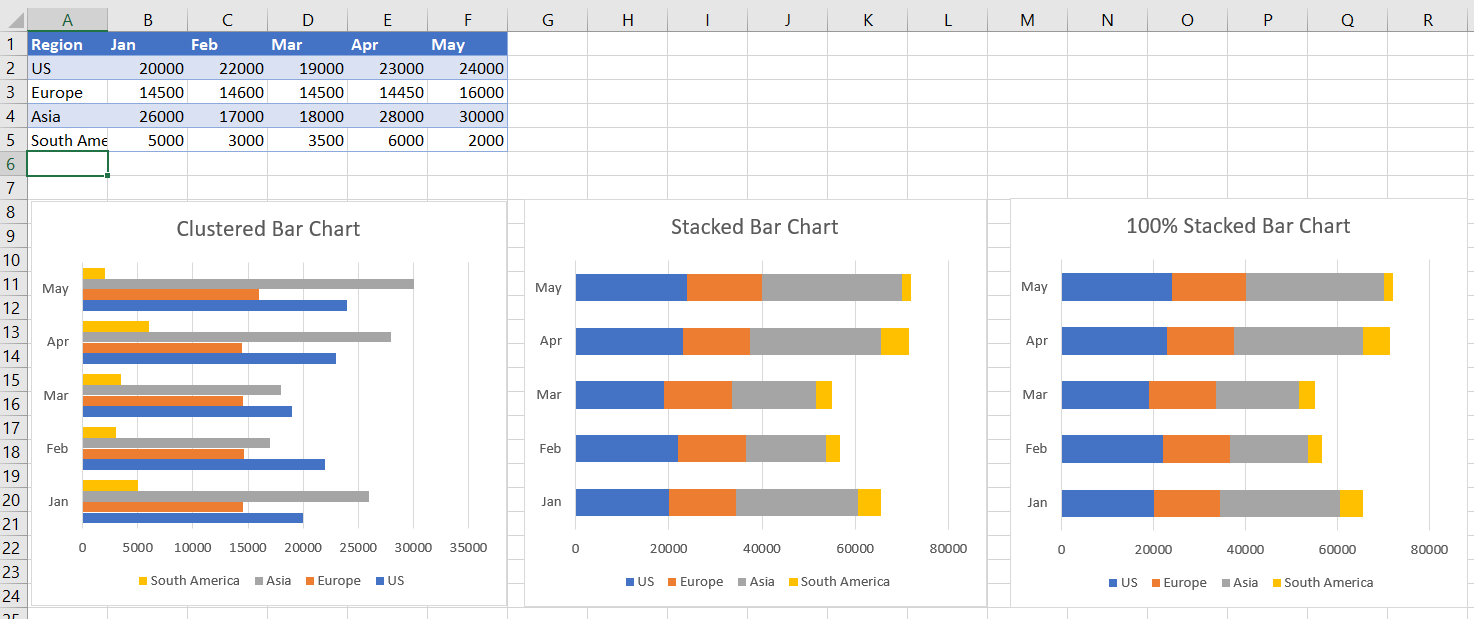
Then head to the Insert tab of the Ribbon. And you can do the following steps to add a vertical line to the horizontal bar chart type in Excel. And select Clustered Bar chart type.
I assume you have a clustered bar chart with horizontal bars. Type your custom number format code into Format Code textbox. Assume you have values of 50 120 and 30 in three cells A1 A2 and A3 and a total of 200 in A4 all in sheet 1 and you then create a stacked bar chart in Sheet 2.
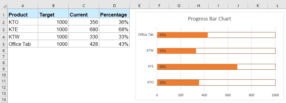
Verified 4 days ago. Select the data range that you want to create a chart but exclude the percentage column and then click Insert Insert Column or Bar Chart 2-D Clustered Column Chart see screenshot. In Excel 2013 or the new version click Design Add Chart Element Data Labels Center.
In the chart right-click the Series Footballers Data Labels and then on the short-cut menu click Format Data Labels. Double-click on the value-axis that you want to modify. As shown below cells A2A5 contain the data Items.
Once your data is selected click Insert Insert Column or Bar Chart. Now a bar chart is created in your worksheet as below screenshot shown. Just click on the map then choose from the Chart Design or Format tabs in the ribbon.
Once your map chart has been created you can easily adjust its design. Layout number 5 is with the Data Table. Now we have a simple Column chart for our data.
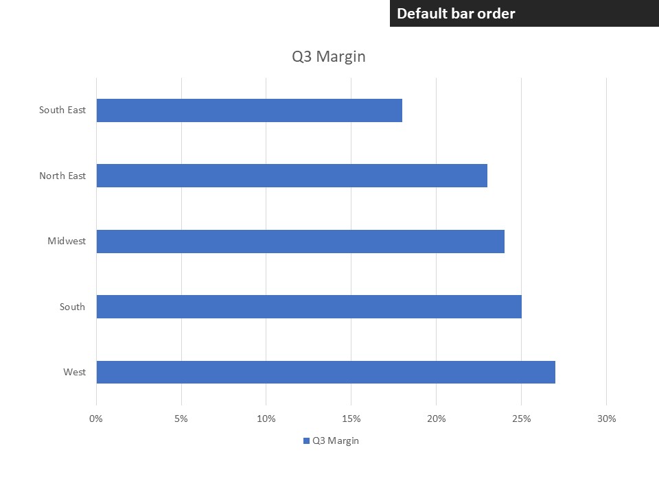
The chart will be inserted for the selected data as below. Select a preset number format or Custom in Category dropdown. 1 select the original data that you want to build a horizontal bar chart.
You can also double-click the chart to launch the Format Object Task Pane which will appear on the right-hand side of the Excel windowThis will also expose the map chart specific Series options see below. Popular Course in this category Excel Advanced Training 14. Cells B2B5 contain the data Values.
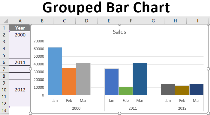
Grouped Bar Chart Creating A Grouped Bar Chart From A Table In Excel
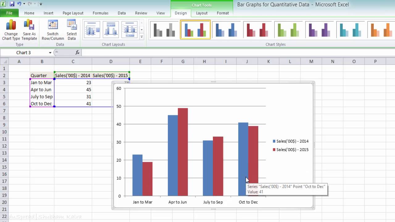
Simple Bar Graph And Multiple Bar Graph Using Ms Excel For Quantitative Data Youtube

Count And Percentage In A Column Chart
How To Add Totals To Stacked Charts For Readability Excel Tactics
How To Create A Stacked Clustered Column Bar Chart In Excel
Add Totals To Stacked Bar Chart Peltier Tech
Making A Simple Bar Graph In Excel Youtube
Bar Chart Target Markers Excel University

Excel Bar Charts Clustered Stacked Template Automate Excel

How To Create A Bar Chart In Excel Displayr
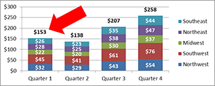
How To Add Total Labels To Stacked Column Chart In Excel
How To Create Progress Bar Chart In Excel

How To Insert In Cell Bar Chart In Excel

How To Create A Bi Directional Bar Chart In Excel
8 Steps To Make A Professional Looking Bar Chart In Excel Or Powerpoint Think Outside The Slide
How To Make A Bar Graph In Excel Clustered Stacked Charts

How To Add Total Labels To Stacked Column Chart In Excel
Ms Excel 2016 How To Create A Bar Chart
Column Chart In Excel Easy Excel Tutorial