How To Add Values To Excel Chart Legend
Add legend to an Excel chart. To remove the legend select None.

Pin On Excel
On the Design tab in the Data group click Select Data.

How to add values to excel chart legend. From the Legend drop-down menu select the position we prefer for the legend. Click on the data chart you want to show its data table to show the Chart Tools group in the Ribbon. Created a Pie Chart and would like to add the data values in the legend as wellie Raws 400 Other 600 Is this poosible.
Locate Select Data on the Design Tab. Change Legend Names Excel. In Excel in the Chart Tools group there is a function to add the data table to the chart.
Here Excel offers a list of handy chart elements. Change Legend Names Excel. Click the chart that displays the legend entries that you want to edit.
Then click on the green plus sign which you can see on the outside of the top right corner of the chart area border. In the Series Name field type a new legend entry. Legend Entry Tricks In Excel Charts Peltier Tech.
In Row 4 enter the formula A1 TextA30 Copy this across. Hi I am trying to add the values and percentages to the legend of a pie chart. Assuming BMW Chevy and Ford are A1-C1 with their values below.
Total value to pie chart legend pie chart microsoft power bi munity doughnut chart total value pie chart in excel how to create pie chart visualization Create Outstanding Pie Charts In Excel Pryor Learning SolutionsShow Or Hide Total Values On A Chart How To Visualizations Doentation LearningCreate Outstanding Pie Charts In Excel Pryor Learning SolutionsCreate. The values from these cells are now used for the chart data labels. Excel Chart Legend How To Add And Format.
Select the stacked column chart and click Kutools Charts Chart Tools Add Sum Labels to Chart. Edit legend entries in the Select Data Source dialog box. Select the source data and click Insert Insert Column or Bar Chart Stacked Column.
Then create a drawing with the colors for the real data series and place it on top of the chart as a secondary legend. Do you know if there is a way to add the values and percentages to the legend of a pie chart in Excel. Then all total labels are added to every data point in the stacked column chart immediately.
Select an entry in the Legend Entries Series list and click Edit. No in your Pie chart. Then delete every series but the gray ones from the legend.
So if I understand correctly Id add two dummy series to the chart with 0 values and assign them dashed and dotted respectively with a neutral gray color. Excel Pie Chart Formatting Inquiry - Trying To Remove Gray Line Within Pie Chart. Click Layout Data Table and select Show Data Table or Show Data Table with Legend Keys option as you need.
In the Select Data Source dialog box. This displays the Chart Tools adding the Design Layout and Format tabs. Copy this across the other columns.
Created a Pie Chart and would like to add the data values in the legend as wellie Raws 400 Other 600 Is this poosible. An example of how I would like it to display is attached. Add Or Remove Labels In A Chart Os Excel.
To move the chart legend to another position select the chart navigate to the Design tab click Add Chart Element Legend and choose where to move the legend. In row 3 enter the formula A2sumA2C2. Excel Charts Add Le Customize Chart Axis Legend And Labels.
If you want to display the legend for a chart first click anywhere within the chart area. Tick the option Legend and Excel will display the legend right away. Select cells C2C6 to use for the data label range and then click the OK button.
The legend will then appear in the. Click Chart Filters next to the chart and click Select Data. Click the Layout tab then Legend.
You can also select a cell from which the text is retrieved. Another way to move the legend is to double-click on it in the chart and then choose the desired legend position on the Format Legend pane under Legend Options. Click anywhere on the chart.
Delete Legend And Specific Entries From Excel Chart In C. I know I can add it to the main area of the chart but because of the number of fields it is very hard to read that way. Select the chart choose the Chart Elements option click the Data Labels arrow and then More Options Uncheck the Value box and check the Value From Cells box.
How to Display the Legend for a Chart.

Pin On Ms Excel

Draw Multiple Overlaid Histograms With Ggplot2 Package In R Example Histogram Overlays Data Visualization

How To Make Awesome Ranking Charts With Excel Pivot Tables Microsoft Excel Tutorial Excel Tutorials Excel Shortcuts

Switch Row And Column Layout In Excel Chart Column Layout The Row

Excel Lesson Activities Excel Tutorials Excel For Beginners Excel
Tech 011 Create A Calendar In Excel That Automatically Updates Colors Excel Calendar Excel Calendar Template Calendar Template

Excel Charts Microsoft Excel Computer Lab Lessons Excel

Pin By Mack Mans On Excel Tutorial Excel Tutorials Chart Labels

Project Status Reporting Show Timeline Of Milestones Change Data Series Chart Type Excel Templates Excel Templates Project Management Book Report Projects

The Datographer Creating A 45 Degree Reference Line In A Tableau Scatter Plot Without Sql Scatter Plot Plot Chart Reference

Pin On Software

Dashboard Creating Sontrol Shart Create A Chart Chart Dashboard
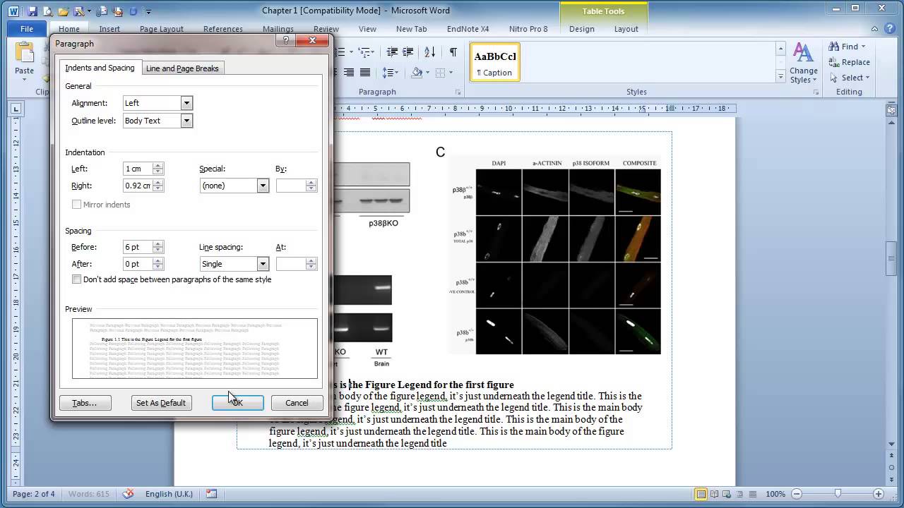
Microsoft Word Inserting Figures And Legends Microsoft Word Document Microsoft Microsoft Word

Show Or Hide Subtotals And Totals In A Pivottable Excel Column Labels

Group Data In An Excel Pivottable Pivot Table Excel Data

Pin By Mack Mans On Excel Tutorial Excel Tutorials Chart Labels

Pin By Tiana T On I Heart Spreadsheets Excel Shortcuts Excel Tutorials Excel Hacks

United Computer Consultants How To Plan And Construct An Excel Spreadsheet Goal Seek And Scenario Manager Excel Data Analysis Tools Excel Spreadsheets
How To Use Filled Map In Excel Map Excel Being Used